Intersystem Noise Coupling
Intersystem Noise Coupling
Overview
The body runs several physiological systems in parallel, cardiac, locomotor, endocrine, neural, and clinical medicine typically studies each in isolation. But none of these systems hold perfectly still: heart rate varies beat to beat, movement intensity fluctuates second to second. That variability isn’t noise in the dismissive sense. It’s structured, and structure shared between two systems is a signal worth measuring directly.
This project models heart rate variability and movement intensity as a pair of coupled Ornstein-Uhlenbeck processes, stochastic differential equations describing how a system relaxes toward equilibrium under continuous random perturbation, and fits the coupling terms between them per subject.
The hypothesis: a healthy body holds a characteristic coupling signature between its systems, one that reorganizes, strengthens, or breaks down under physiological stress or disease.
Method
Signal extraction — RR intervals from ECG for the cardiac signal, accelerometer magnitude (√x²+y²+z²) for the locomotor signal, both resampled onto a shared 4 Hz grid so the two are directly comparable.
Frequency-domain analysis — power spectral density of heart rate variability, split into low-frequency (0.04–0.15 Hz) and high-frequency (0.15–0.40 Hz) bands, with their ratio used as an index of sympathovagal balance.
Cross-organ coherence — spectral coherence between the cardiac and locomotor signals, to identify which frequencies, if any, the two systems synchronize at.
Coupled OU model fitting — the core model:
dX = θ_x(−X)dt + κ_xy·Y·dt + σ_x·dW_x    (cardiac)
dY = θ_y(−Y)dt + κ_yx·X·dt + σ_y·dW_y    (locomotor)
κ_xy and κ_yx capture directional coupling strength — locomotion→cardiac and cardiac→locomotion respectively — σ_x and σ_y the intrinsic noise level of each system, θ_x and θ_y how fast each reverts to its own baseline. Parameters are fit per subject by least-squares regression on the discretized derivatives.
Transfer entropy — a model-free, information-theoretic check on the same question: how much knowing one system’s past reduces uncertainty about the other’s future, without assuming the linear relationship the OU model does.
Windowed coupling — the same OU fit repeated across sliding windows within a single recording, to test whether coupling is a fixed trait or something that shifts over the course of a day.
Phase One: The Healthy Baseline
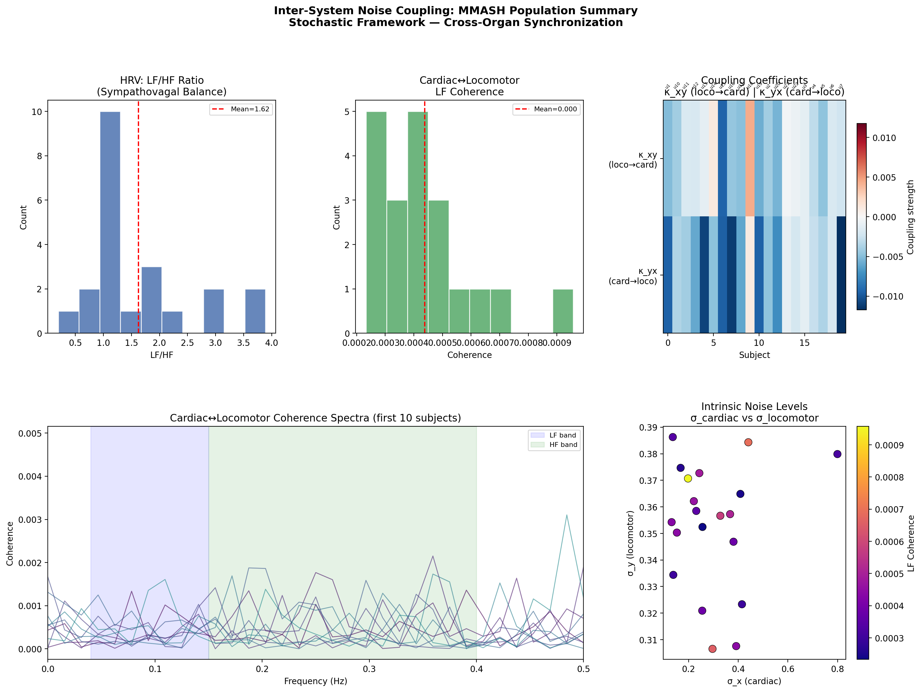
MMASH 24-hour continuous ECG and wrist-accelerometer recordings from 20 healthy, active adults, establishes what an undisturbed, healthy pair of systems looks like.
| Metric | Value | Interpretation |
|---|---|---|
| Mean LF/HF ratio | 1.62 | Slight sympathetic dominance, normal for an active cohort |
| Mean LF coherence | ~0.000 | Cardiac and locomotor systems are largely independent |
| Mean κ_xy (loco → cardiac) | −0.00551 | Movement mildly suppresses cardiac variability |
| Mean κ_yx (cardiac → loco) | −0.00076 | Cardiac activity barely influences movement |
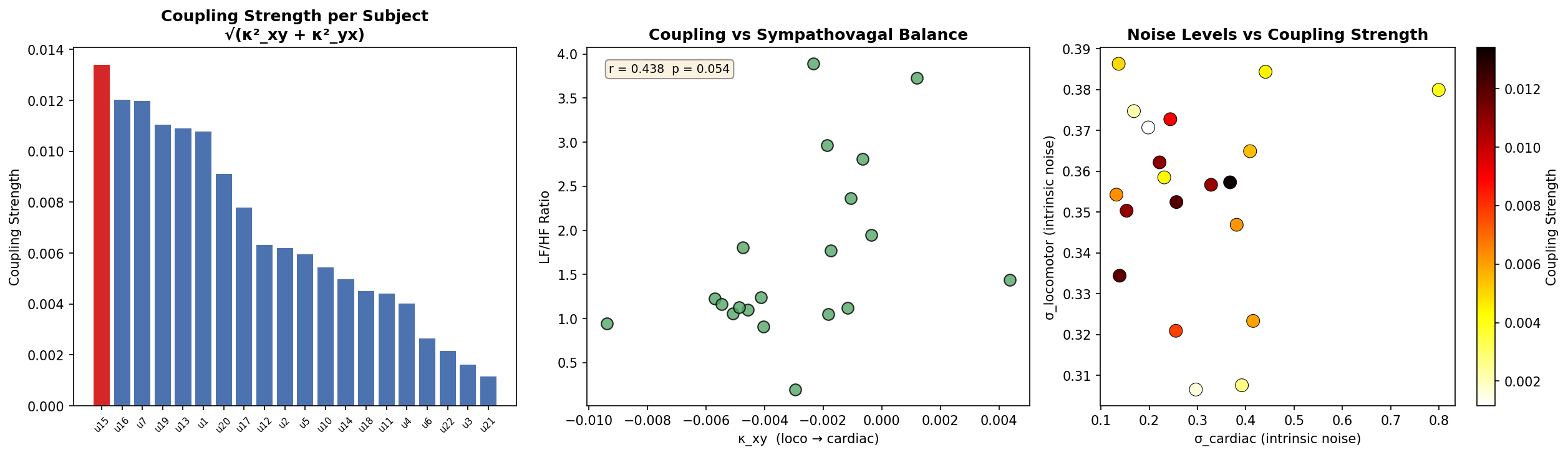
| κ_xy vs. LF/HF correlation | r = 0.436, p = 0.054 | A trend, just short of conventional significance: more coupling tracks with more sympathetic activation |
| σ_cardiac range | 0.13 – 0.80 | Cardiac noise varies substantially between people |
| σ_locomotor range | 0.31 – 0.39 | Locomotor noise is remarkably consistent across people |
The pattern in healthy people is near-independence, not synchrony — and the small coupling that does exist is negative: movement quiets cardiac variability, consistent with vagal withdrawal during physical activity.
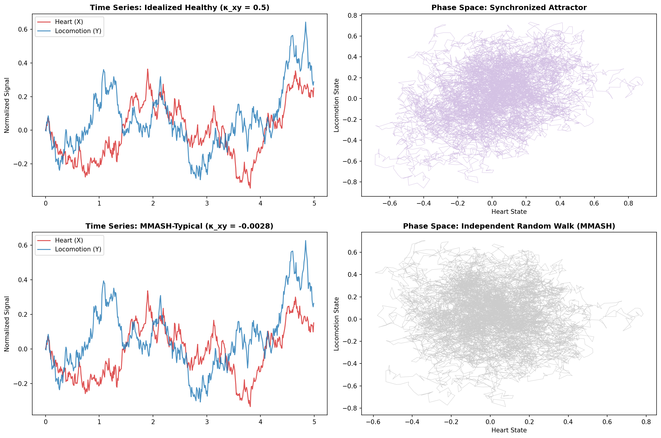
One subject stands apart from this pattern entirely, showing anomalously positive coupling on every metric — a single, consistent outlier rather than noise in the fit.
Phase Two: Testing It Under Stress
The healthy baseline is the control condition, not the finding. The actual test of the hypothesis is whether this near-independence signature holds up when a system is under genuine physiological strain — and that’s what MIMIC-IV is for. ICU waveform data (ECG-derived RR intervals and respiratory waveforms from critically ill patients) will run through the identical pipeline, asking directly: does intersystem coupling strengthen, reorganize, or break down under critical illness? That comparison is what turns this from a description of healthy physiology into a candidate diagnostic signature.
Key tools: Python · NumPy · SciPy · Stochastic differential equations · Transfer entropy